Guidance is becoming a cheat code for LLMs (with Loooop)
Guidance can dramatically improve prompt following and sample quality in image and video generation, simply by changing how a trained model is sampled.1 Classifier-free guidance (CFG) is a standard ingredient in Stable Diffusion 32 and Wan3. Its benefits are valuable enough that FLUX.1 [dev] is trained to distill guidance directly into the model.4
Can language models benefit in the same way? There is a catch: applying guidance to each next-token prediction does not generally produce the desired guided joint distribution over the full token sequence. The two procedures normalize probabilities differently. Looped models offer a way to narrow this gap.11, 12, 16, 23 When predictions from different loops are close, guidance changes token preferences at first order, while the normalization error enters at second order. In this blog, we explain why loops can make guidance more natural for language models, and how this connects them to diffusion.
01Why diffusion guidance needs no normalizer

Start with a conditional density \(p(x\mid c)\), where \(c\) might be a text prompt. Suppose we want to favor samples that are especially characteristic of that condition. One way to express this preference is to tilt the density:
The ratio \(p(x\mid c)/p(x)\) favors samples that are more likely under the prompt than without conditioning. At \(w=0\), we recover ordinary conditional generation. Increasing \(w\) strengthens that preference. The normalizer \(Z_w(c)\) makes the density integrate to one.
Diffusion models use the score, the gradient of a log density, to guide denoising. Following common practice, we compute the score without knowing the normalizer, as the normalizer \(Z\) is considered independent of \(x\)5. Guidance can therefore be written as a combination of the conditional and unconditional scores:
This is the score combination behind classifier-free guidance1. In this score formulation, the normalizer vanishes.*
02Token-level guidance and the joint distribution

Guidance already exists in autoregressive LLMs. Stay on topic with Classifier-Free Guidance8 applies CFG by contrasting next-token predictions with and without the conditioning prompt, while keeping the generated prefix. Contrastive decoding9 uses a weaker model as the reference; DoLa10 uses predictions from earlier layers. Here we study their shared core idea: combine two next-token predictions, then normalize.
The joint distribution assigns a probability to every complete token sequence. Applying guidance to that distribution means reweighting each sequence and normalizing once. Token-level guidance instead normalizes separately at each prefix. These operations generally produce different sequence probabilities.
As Sander noted in his 2022 blog post:
“my hunch is that diffusion guidance works so well precisely because we are able to apply it to the joint distribution”
Let \(p_K\) be the predictor we want to strengthen and \(p_E\) its reference. For a sequence \(y=(y_1,\ldots,y_T)\) of fixed length \(T\), \(y_t\) is the next token and \(y_{<t}=(y_1,\ldots,y_{t-1})\) is its prefix. Assuming positive token probabilities and leaving the fixed prompt conditioning implicit, token-level guidance gives
Here \(C(y_{<t})\) is the local normalizer; the sum runs over all possible next tokens.
Write \(p_K(y)\) and \(p_E(y)\) for each model's sequence probability, obtained by multiplying its token probabilities. The guided joint distribution uses a single global normalizer \(Z\); token-level guidance instead multiplies the locally normalized probabilities \(q\):
The numerators are identical, but the normalizers differ: \(Z\) is shared by every sequence, whereas the product of local normalizers depends on the sequence's prefixes \(y_{<t}\). This is the normalization mismatch.
Additionally, computing the full-sequence normalizer \(Z\) exactly is impractical for real LLMs: it requires summing over all possible future token sequences, whose number grows exponentially with length.
If the guided joint distribution is our target, practical token-level guidance therefore tolerates a normalization error. The local rule avoids summing over future sequences by normalizing only the next-token scores. The question is how to make the resulting error small.
A tiny example makes the difference visible
Suppose a sequence has just two tokens. Both predictors choose \(A\) or \(B\) with probability \(1/2\). After \(A\), both remain uniform over \(1,2\). After \(B\), the reference is still uniform but the stronger predictor assigns probabilities \(0.9,0.1\). Token-level guidance cannot change the first decision: the predictors agree there. The guided joint distribution can, because it accounts for the guided weight of the continuations after \(B\).
Same token weights, different sequence probabilities
Compare token-level \(Q_{\rm local}\) with the joint target \(Q_{\rm joint}\) from Equation (3). If they were equivalent, they would give the same probability of starting with B. Shrink the predictor difference to see the gap close.
Probability of starting with B
\(Q_{\rm local}\)
\(Q_{\rm joint}\)
12.1 percentage-point gap. Even the first-token probabilities differ.
03Loooop

A looped Transformer applies the same block of layers repeatedly before predicting the next token. Huginn11 and Ouro12 implement this idea in different ways. Each completed loop gives a hidden state that can be converted into next-token logits (unnormalized token scores): \(z_E\) after an earlier loop \(E\), and \(z_K\) after the final loop \(K\).
The earlier prediction serves as the weaker reference for guiding the final prediction. Both come from the same model on the same text prefix; the difference is how many loops of computation they use.
LoopCD13 uses these predictions for guidance without additional training. Its logit variant strengthens the final logits \(z_K\) along the difference \(z_K-z_E\). Applying softmax gives \(q\), the guided next-token probability distribution:
LoopCD's logit variant uses the first loop as its reference. The paper also combines hidden states before converting them into logits; the analysis below concerns the logit rule in Equation (4).

Because every loop repeats the same computation, its predictions are expected to stay close as the hidden state is refined. This gives us a route back to the normalization problem: close loop predictions can make token-level guidance a better approximation to the guided joint distribution. Below we show how the error depends on their logit difference, then measure that difference.
Why loops help
The key assumption is that predictions from different loops have similar logits. Under this small-difference assumption, we can bound the local normalizer \(C(y_{<t})\).
At a fixed prefix, write \(\delta=z_K-z_E\). After removing an irrelevant constant offset, assume \(\delta=\epsilon d\), with \(d\) bounded and \(\epsilon\) small. Keep the guidance strength fixed and bounded. A Taylor expansion gives
The constant and first-order terms cancel. Guidance changes token log-odds at first order; its local log-normalization cost starts at second order.
Proof of Equation (5)
Fix a prefix \(y_{<t}\). The local normalizer satisfies the exact identity
Proof of Equation (6). For each possible next token \(y_t\), rearrange the definition of \(q(y_t\mid y_{<t})\):
Taking the expectation over \(y_t\sim p_K(\cdot\mid y_{<t})\) yields Equation (6). For \(w\geq0\), both KL terms are nonnegative, so \(\log C(y_{<t})\geq0\). This identity does not require small logit differences. \(\square\)
For the Taylor expansion, write the logit difference as \(\delta(y_t\mid y_{<t})=z_K(y_t\mid y_{<t})-z_E(y_t\mid y_{<t})\). Define its log moment-generating function under the reference distribution:
Softmax gives
Substituting into the definition of \(C(y_{<t})\), we obtain the exact expression
For \(\delta=\epsilon d\) with uniformly bounded \(d\), and bounded \(\alpha\), expand
The expectation and variance are over next tokens \(y_t\) at the same prefix \(y_{<t}\). Substitution cancels the linear terms and leaves
This proves Equation (5). \(\square\)
Suppose \(0\leq\log C(y_{<t})\leq\eta\) at every prefix of a length-\(T\) sequence. Equation (3) then bounds the log-probability difference between token-level guidance and the guided joint distribution:
Equation (7) bounds the full-sequence error by \(T\eta\). Under the uniform small-difference assumption, \(\eta=O(\epsilon^2)\), so this error is \(O(T\epsilon^2)\): close predictions let the token-level rule approximate the guided joint distribution without summing over future sequences.
Proof of Equation (7)
Set \(D(y)=\prod_t C(y_{<t})\). Equation (3) gives \(ZQ_{\rm joint}(y)=Q_{\rm local}(y)D(y)\). Summing over sequences gives
The prefix bound gives \(1\leq D(y)\leq e^{T\eta}\) for every sequence. Its expectation obeys the same bounds, so \(0\leq\log Z\leq T\eta\). Finally,
Both terms lie in \([0,T\eta]\), establishing Equation (7). This argument retains the global normalizer rather than dropping it.
This is why similar loop outputs help: guidance changes token preferences at first order in \(\epsilon\), while the mismatch between token-level guidance and the guided joint distribution is \(O(T\epsilon^2)\) for a sequence of length \(T\).
04Are predictions from different loops actually closer?
We compared two looped models, Huginn-0125 and Ouro-2.6B, with two ordinary Transformers, Qwen2.5-3B and Pythia-2.8B. Each model saw the same 1,024 text prefixes: eight positions on each of 128 GSM8K development questions. At each prefix, we compared the model's next-token logits partway through its computation with its own final logits.
Here, depth \(k\) means the number of completed loops in a looped model, or completed layers in an ordinary Transformer. The final depth \(K\) stays fixed. Let \(V\) be the vocabulary size and \(v\in\{1,\ldots,V\}\) a candidate token's index. Then \(z_{k,v}(y_{<t})\) is that token's score after depth \(k\), on the same text prefix \(y_{<t}\).
For each \(k\), compute the change to the final score, \(\delta^{(k)}_v(y_{<t})=z_{K,v}(y_{<t})-z_{k,v}(y_{<t})\). Remove its vocabulary mean, \(\bar\delta^{(k)}(y_{<t})=V^{-1}\sum_v\delta^{(k)}_v(y_{<t})\), because adding the same constant to every logit does not change softmax. We measure the remaining change with
Intuitively, this measures how much the next-token scores change between an intermediate depth and the final depth. It is the standard deviation of those score changes across the vocabulary. A smaller value means the predictions vary less as the model performs more loops or layers.
In the plot, we vary \(k\), keep the prefix and final depth \(K\) fixed, and average the RMS over the 1,024 prefixes. The horizontal position is \(k/K\): 50% means halfway through that model. The depths used for the quarter, half, and three-quarter comparisons are:
| Model | Intermediate \(k\): 25%, 50%, 75% | Fixed final \(K\) |
|---|---|---|
| Huginn-0125 | Loops 8, 16, 24 | 32 loops |
| Ouro-2.6B | Loops 1, 2, 3 | 4 loops |
| Qwen2.5-3B | Layers 9, 18, 27 | 36 layers |
| Pythia-2.8B | Layers 8, 16, 24 | 32 layers |
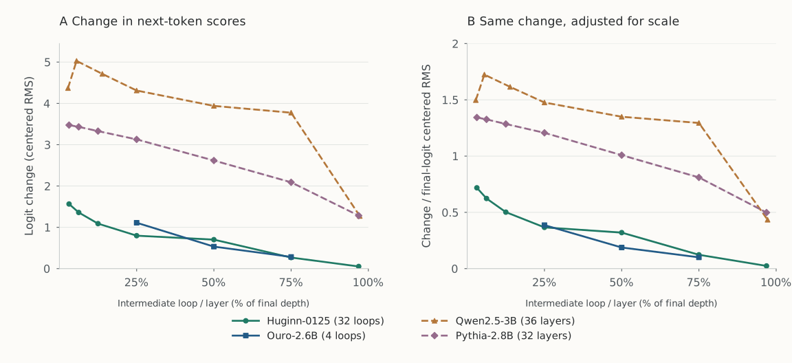
The looped models' mean gaps are 2.8–14.1 times smaller across all twelve comparisons. Every paired 95% bootstrap interval for the ratio lies below one. The ordering also holds after scale normalization and when using only question prefixes, before any answer text.
The smaller logit gaps support the proposed mechanism: loop predictions stay closer, making smaller normalization errors plausible. Under the small-difference assumption, guidance changes token preferences at first order while the normalization error grows only at second order. This gives looped models a natural route toward effective token-level guidance that stays close to the desired joint distribution.
05Loops and diffusion, beyond guidance

Guidance is one connection between looped models and diffusion; learning to refine a prediction is the broader one. Autoguidance uses a smaller, less-trained diffusion model as a reference,14 while a looped model can use its own earlier prediction. In both cases, a weaker prediction provides information for improving a stronger one.
These connections are now explicit in the methods themselves. Time-Modulated Looped Transformers15 borrow diffusion-style timestep conditioning, and LoopFormer16 adds step-size conditioning and shortcut consistency. Denoising Recursion Models17 learn multi-step correction of corrupted solutions, while Thinking with Looped Flows18 couples recurrent states to a learned denoising flow. In the other direction, Looped Diffusion Language Models19 and Looped-DiT20 repeat Transformer blocks inside diffusion models, allowing compute to grow through loop depth as well as sampling steps.
Test-time-scaling work suggests a sharper perspective: capability depends on how computation is organized, not only on how much is spent.21 Both looped models and diffusion offer test-time scaling through iterative refinement, spending extra computation on hidden-state updates or sampling steps. Their connection is not just that they repeat computation, but that the inference algorithm determines how those updates are used: how many to take, how large they should be, and how guidance steers them. What scales is the model together with its inference algorithm.
* Score-based models learn scores of noisy distributions from samples.22 Combining conditional and unconditional score estimates implements the reweighting idea at each noise level, although the resulting sampler need not reproduce the corresponding clean-data distribution in Equation (1).5,6,7 We therefore view score-level CFG as a practical surrogate for distribution-level reweighting. ↩
References
- Jonathan Ho and Tim Salimans. Classifier-Free Diffusion Guidance. arXiv, 2022. ↩1 ↩2
- Patrick Esser et al. Scaling Rectified Flow Transformers for High-Resolution Image Synthesis. ICML, 2024. ↩
- Wan Team. Wan: Open and Advanced Large-Scale Video Generative Models. arXiv, 2025. ↩
- Black Forest Labs. FLUX.1 [dev]. Model card, 2024. ↩
- Sander Dieleman. Guidance: a cheat code for diffusion models. May 26, 2022; including the May 29 correction. ↩1 ↩2 ↩3
- Arwen Bradley and Preetum Nakkiran. Classifier-Free Guidance is a Predictor-Corrector. arXiv, 2024. ↩
- Muthu Chidambaram et al. What does guidance do? A fine-grained analysis in a simple setting. arXiv, 2024. ↩
- Guillaume V. Sanchez et al. Stay on topic with Classifier-Free Guidance. arXiv, 2023. ↩
- Xiang Lisa Li et al. Contrastive Decoding: Open-ended Text Generation as Optimization. arXiv, 2022. ↩
- Yung-Sung Chuang et al. DoLa: Decoding by Contrasting Layers Improves Factuality in Large Language Models. arXiv, 2023. ↩
- Jonas Geiping et al. Scaling up Test-Time Compute with Latent Reasoning: A Recurrent Depth Approach. arXiv, 2025. ↩ ↩1
- Rui-Jie Zhu et al. Scaling Latent Reasoning via Looped Language Models. arXiv, 2025. ↩ ↩1
- Weihao Liu et al. Decoding Looped Transformers Better for (Almost) Free. arXiv, 2026. ↩1 ↩2
- Tero Karras et al. Guiding a Diffusion Model with a Bad Version of Itself. NeurIPS, 2024. ↩
- Kevin Xu and Issei Sato. On Expressive Power of Looped Transformers: Theoretical Analysis and Enhancement via Timestep Encoding. ICML, 2025. ↩
- Ahmadreza Jeddi, Marco Ciccone, and Babak Taati. LoopFormer: Elastic-Depth Looped Transformers for Latent Reasoning via Shortcut Modulation. arXiv, 2026. ↩ ↩1
- Chris Cameron et al. One Step Forward and K Steps Back: Better Reasoning with Denoising Recursion Models. arXiv, 2026. ↩
- Ayhan Suleymanzade, Chanhyuk Lee, Floor Eijkelboom, Nicholas M. Boffi, İsmail İlkan Ceylan, and Jinwoo Kim. Thinking with Looped Flows. arXiv, 2026. ↩
- Sanghyun Lee et al. Looped Diffusion Language Models. arXiv, 2026. ↩
- Yong Xien Chng et al. Looped Diffusion Transformer. arXiv, 2026. ↩
- Edward Beeching, Lewis Tunstall, and Sasha Rush. Scaling test-time compute with open models. Hugging Face, 2024. ↩
- Yang Song et al. Score-Based Generative Modeling through Stochastic Differential Equations. ICLR, 2021. ↩
- Benhao Huang et al. Towards Looped Models Done Right, Part II: Rethinking at Fixed Points. arXiv, 2026. ↩